MLA programming
The MLA™ comes with a Python software interface consisting of two main parts:
MLA API (Application Programming Interface) is a software library for accessing the MLA™ hardware, set up and control of measurements with the MLA™, and reading out the measurement data from the MLA™.
MLA GUI (Graphical User Interface) is a versatile interface for setting up and performing many different types of measurements with the MLA, plotting the results, and saving the data to the computer for further analysis.
Thanks to Python’s interactive environment it is possible to use the MLA API directly from the Python command line. Command line statements can be bunched together into scripts for automated set up and measurement. Such scripts could then be run stand-alone, integrated into other software, or run from the script panel built in to the MLA GUI. The same API is used in all cases and it serves as the foundation for full-featured interactive graphical applications, such as the MLA GUI.
The MLA GUI can be used entirely without programming, but many tasks are still best performed by scripting. Therefore, a Python shell panel for running single Python commands, and a Script panel for writing and executing Python scripts, is available inside the MLA GUI. The combination of a GUI and programming capability in the same application can be very practical in many situations. For example, you can use the Oscilloscope panel and the Lockin plot panel for debugging your measurement setup. When all looks fine, you can start your script which performs the measurement, data analysis and plotting. The MLA GUI includes a rich set of built-in scripts that can be used as templates for your custom scripts.
There are many options for programing the MLA™, but no matter which option you choose, you use the same MLA API, so that all MLA™ commands look exactly the same. You can test your commands in the Python shell panel and the move them over to the Script panel. When you are building a larger a stand-alone measurement script, you use the Script panel in the MLA-GUI to test and debug pieces of code, and then paste the code into your stand-alone script.
NumPy and matplotlib
The MLA software uses the open-source libraries NumPy for array math and matplotlib for plotting. Together, NumPy and matplotlib provide an experience much similar to the well-known MATLAB © software. Both NumPy and matplotlib are well documented on their respective web pages. In particular the matplotlib gallery is very useful. If you are familiar with MATLAB ©, a quick way to get started would be to read NumPy for MATLAB users .
In the code samples of this user manual, and in the built-in scripts that are provided with the MLA software, we use the convention that all NumPy commands start with np., as in y = np.sin(x) because we import numpy as np. Similarly, matplotlib commands can start with plt. as in plt.plot(x,y) because we import matplotlib.pyplot as plt. But with matplotlib we often generate new objects, and work with their member functions, as in the sequence:
import numpy as np
import matplotlib.pyplot as plt
x = np.linspace(0,2*np.pi)
y = np.cos(x)
fig = plt.figure()
ax1 = fig.add_subplot(2,1,1)
ax1.plot(x,y)
plt.draw()
plt.show()
When running integrated MLA scripts matplotlib.pyplot sometimes uses a conflicting GUI back-end, resulting in the rest of the MLA GUI freezing while the figure is displayed. To avoid this problem, plotting can instead be done inside the MLA GUI, from the Script plot panel or Pyhton shell panel, using the scriptplot object, as demonstrated in the example below.
x = np.linspace(0,2*np.pi)
y = np.cos(x)
fig = scriptplot.fig
ax1 = fig.add_subplot(2,1,1)
ax1.plot(x,y)
wx.CallAfter(scriptplot.my_draw)
For more details on script plotting inside the GUI, see plotting in the GUI.
MLA API
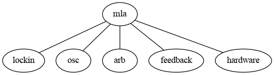
The Application Programming Interface (API) for the MLA is the main object which we always instantiate with the name mla in Python code. This API object is a container with five basic singleton objects.
Complete documentation of all the member functions of each class is found under the links below.
- mla
- mla.lockin
LockinLockin.abort_parameter_sweep()Lockin.abort_wait_for_counter()Lockin.abort_wait_for_new_pixels()Lockin.abort_wait_for_trigger()Lockin.arm_trigger()Lockin.blank_output()Lockin.enable_pixel_clock()Lockin.enable_wait_for_trigger()Lockin.extract_dc()Lockin.flush_trigger_queue()Lockin.frequency_sweep()Lockin.frequency_sweep_multifreq()Lockin.get_Tm()Lockin.get_Tm_max()Lockin.get_Tm_min()Lockin.get_amplitudes()Lockin.get_counter()Lockin.get_da_max()Lockin.get_da_min()Lockin.get_df()Lockin.get_df_max()Lockin.get_df_min()Lockin.get_frequencies()Lockin.get_frequency_sweep()Lockin.get_frequency_sweep_multifreq()Lockin.get_fsample()Lockin.get_input_multiplexer()Lockin.get_line()Lockin.get_new_pixels()Lockin.get_parameter_sweep()Lockin.get_phases()Lockin.get_pixel_average()Lockin.get_pixels()Lockin.get_pixels_between_bufpos()Lockin.get_port()Lockin.get_samples_per_pixel()Lockin.get_samples_per_pixel_max()Lockin.get_samples_per_pixel_min()Lockin.get_tone()Lockin.is_started()Lockin.line_up_phases()Lockin.load_from_file()Lockin.logger_start()Lockin.logger_stop()Lockin.measure_packet_rate()Lockin.reset_outputs()Lockin.reset_tones_on_new_pixel()Lockin.reset_tones_on_trig1()Lockin.save_to_file()Lockin.send_trigger()Lockin.set_Tm()Lockin.set_amplitudes()Lockin.set_dc_offset()Lockin.set_df()Lockin.set_digital_mask()Lockin.set_frequencies()Lockin.set_frequencies_by_n_and_df()Lockin.set_input_multiplexer()Lockin.set_output_mask()Lockin.set_output_mode_lockin()Lockin.set_phases()Lockin.set_samples_per_pixel()Lockin.set_trigger_flanks()Lockin.set_trigger_in_flank()Lockin.set_trigger_in_holdoff()Lockin.start_lockin()Lockin.start_parameter_sweep()Lockin.start_parameter_sweep_native()Lockin.stop_lockin()Lockin.tune0()Lockin.tune1()Lockin.tune2()Lockin.wait_for_counter()Lockin.wait_for_new_pixels()Lockin.wait_for_settings_effect()Lockin.wait_for_trigger()
LockinReceiver
- mla.osc
- mla.arb
- mla.feeback
FeedbackFeedback.activate_phase()Feedback.afm_engage()Feedback.afm_lift()Feedback.autosetup_afm()Feedback.calculate_feedback_amplitude()Feedback.set_current_phase_to_value()Feedback.set_feedback_type()Feedback.set_feedback_type_on_correct_port()Feedback.set_feedback_type_on_port()Feedback.set_feedback_type_slow()Feedback.set_phase_offset()Feedback.setup()
- mla.hardware
HardwareHardware.configure_clk_status_ld()Hardware.configure_memory()Hardware.echo()Hardware.get_firmware_version()Hardware.get_hardware_revision()Hardware.get_input_relay()Hardware.get_nr_freqs_in()Hardware.get_nr_freqs_out()Hardware.get_nr_input_ports()Hardware.get_output_relay()Hardware.get_overflow()Hardware.get_serial_number()Hardware.get_temperature()Hardware.has_relays()Hardware.reset_overflow()Hardware.set_LED()Hardware.set_ad_clock_divisor()Hardware.set_ad_clock_phase()Hardware.set_clkin_parameters()Hardware.set_clkout_divisor()Hardware.set_clkout_power()Hardware.set_clkout_type()Hardware.set_clkref_external_10MHz()Hardware.set_clkref_internal()Hardware.set_dac_auxdac()Hardware.set_dac_clock_divisor()Hardware.set_dac_fsc()Hardware.set_dac_interpolation()Hardware.set_input_relay()Hardware.set_output_multiplexer()Hardware.set_output_relay()Hardware.set_output_type()Hardware.set_slowad_clock_divisor()Hardware.set_slowdac()Hardware.set_slowdac_toggle()Hardware.upload_calibration()Hardware.wait_for_idle()
MLA GUI
The Graphical User Interface (GUI) for the MLA has a Python shell panel and a Script panel from which you can execute all commands in the MLA API. But it is also possible to control the MLA GUI itself from a Python script. For example, you can program the GUI to:
Set which panels should be visible, and their size and position
Control GUI objects such as text fields and check boxes
Configure the plots
The MLA GUI is controlled through it’s hierarchy of objects. At the top level there is the main controller, called main. There is also mla_globals, which is a container for global variables, and the mla object itself. Only a selected subset of the full MLA GUI programming interface is documented under the links below. If you need to access a function that is not documented here, please contact Intermodulation Products.
example scripts
Here follows some examples scripts which can be run from the script panel in the MLA GUI. They serve as starting points for designing your own measurement scripts. These examples are available in the settings/mla_scripts/built-in folder in the user folder.
In every script the MLA API is instantiated as the Python object called mla and all commands are accessed in the code with the form mla.comand.
All commands used in these scripts are documented in detail in MLA API
setup the GUI
Panels can automatically be displayed or hidden using scripts. Most panels are accessed through the main. object. A script can obtain its own filename with __scriptfile__.
# Built-in script. Use the "Save as" button and save under a different filename before editing.


# Set which panels should be visible
main.gui.show_panel(main.scriptpanel)
main.gui.show_panel(main.scriptplot)
main.gui.show_panel(main.shell)
main.gui.show_panel(main.message_log, pos=('Dock()', 'Bottom()', 'Layer(1)'))
main.scriptpanel.open_file(__scriptfile__)
plotting in the GUI
Plotting uses matplotlib and the script plot panel. A pre-existing Figure object is first obtained from scriptplot.fig after which regular matplotlib syntax is used. To draw the figure on the screen the function scriptplot.draw has to be called. As wxPython only allows the main thread to perform to access the GUI this command has to be queued in the main loop using wx.CallAfter. Failure to do so can lead to unstable behavior and crashing of the software.
# Built-in script. Use the "Save as" button and save under a different filename before editing.

# Perform plotting in the Script Plot panel and save the
# resulting figure under an automatically generated filename


fig = scriptplot.fig
fig.clear()

ax = fig.add_subplot(1, 1, 1)
ax.set_xlabel('x')
ax.set_ylabel('t')
ax.set_title('Figure 1')
t = np.linspace(0, 1, 1000)
y = np.sin(2 * np.pi * t)
line = ax.plot(t, y, 'r')[0]

fig.tight_layout()
filename = scriptutils.generate_filename() + '.png'
wx.CallAfter(scriptplot.draw)
wx.CallAfter(fig.savefig, filename)
configuring the lockin
This script demonstrates configuring the lockin using explicit lists. Python lists as well as numpy arrays can be used as an argument when setting properties such as frequency, amplitude and phase. If the length of the argument is less than the number of available tones (i.e. mla.lockin.nr_output_freq()) that property will be set to zero for the remaining, unspecified, tones.
# Built-in script. Use the "Save as" button and save under a different filename before editing.


# Configure lockin
freqs = [10000, 10100, 10200]  # Hz
df = 100  # Hz
phases = [0, 90, 180]  # degree
ampls = [0.01, 0.02, 0.03]  # V
out_1_mask = [1, 1, 1]
out_2_mask = 0

# Tune frequencies
freqs_tuned, df_tuned = mla.lockin.tune1(freqs, df)

# Program MLA
mla.reset()
mla.lockin.set_output_mask(out_1_mask, port=1)
mla.lockin.set_output_mask(out_2_mask, port=2)
mla.lockin.set_phases(phases, 'degree')
mla.lockin.set_amplitudes(ampls)
mla.lockin.set_frequencies(freqs_tuned)
mla.lockin.set_df(df_tuned)
lockin measurement loop
This example takes a lockin measurement and displays the amplitudes in a continuously updating figure. The measurement is running an infinite loop which is broken by changing the Boolean scriptpanel.is_running. The value of this variable will change when the user clicks the Run/Stop button in the Script panel.
The Boolean scriptplot.is_drawing is automatically set to False when scriptplot.draw finishes. If a previous plot was not finished, plotting is skipped to ensure that the GUI remains responsive and the computer is not overloaded with plot requests. To speed up plotting the command ax.plot should be avoided in the loop as this command redraws all axes and ticks etc. Rather, update only the data in an existing matplotlib line.
# Built-in script. Use the "Save as" button and save under a different filename before editing.


freqs = mla.lockin.get_frequencies()

fig = scriptplot.fig
fig.clear()
ax = fig.add_subplot(1, 1, 1)
line = ax.plot(freqs * 1e-3, np.zeros_like(freqs), 'x')[0]
ax.set_xlabel('Frequency (kHz)')
ax.set_ylabel('Amplitude ({})'.format(mla.convert.get_AD_unit()))
fig.tight_layout()

mla.lockin.start_lockin()
while True:
    mla.lockin.wait_for_new_pixels(1)
    pixels, meta = mla.lockin.get_pixels(1)
    if not scriptplot.is_drawing:
        scriptplot.is_drawing = True
        line.set_ydata(np.abs(pixels))
        wx.CallAfter(scriptplot.draw)
    if not scriptpanel.is_running:
        break
mla.lockin.stop_lockin()
frequency sweep
He we demonstrate changing a parameter in a measurement loop. The lockin frequency is stepped through an array f_hz of specified values. After tuning, each value of the bandwidth is set using the command mla.lockin.set_df(df, wait_for_effect=False), followed by the command mla.lockin.set_frequencies(f, wait_for_effect=True). Python does not have to wait for the MLA to reply before it goes on to the second configuration command. However, Python should wait after the last configuration command (i.e. wait_for_effect=True) before it goes on to get new data from the MLA. This speeds up configuration, while ensuring that the configuration is actually in effect when the measurement data is collected.
Note that the lockin is started with the command mla.lockin.start_lockin(cluster_size=1), specifying that only one lockin data packet is sent with each Ethernet package. This speeds up the loop by reducing the latency between the end of measurement and transfer to the computer. The feature is useful when we are interested in fast update after only one lockin measurement. However, a small cluster size will reduce the total bandwidth when a data stream of many lockin measurements is desired.
This example demonstrates stepping any lockin parameters. A frequency sweep is most easily done in the MLA GUI using the frequency sweep panel. In your own scripts, use the function lockin.Lockin.frequency_sweep(), which is optimized for speed, and has the option for multifrequency sweeping is available.
# Simple frequency sweep using Python loop to step through parameters and call MLA commands

# User parameters
f_khz = np.linspace(1, 10000, 1001)
df = 1000.
drive_amp = 0.1

# Setup MLA
mla.lockin.set_df(df)
mla.lockin.set_amplitudes(drive_amp)
mla.lockin.set_output_mask(1, port=1)

# Allocate memory for result
amps = np.zeros_like(f_khz)
amps[:] = np.NAN
phases = np.zeros_like(f_khz)
phases[:] = np.NAN

# Setup GUI
main.gui.show_panel(main.scriptplot)

# Initialize plots
scriptplot.fig.clear()  # remove if you want multiple sweeps in one plot

ax = scriptplot.fig.add_subplot(2, 1, 1)
ax.set_xlabel('Frequency [kHz]')
ax.set_ylabel('Amplitude [V]')
ax.set_title('Frequency sweep')
ax.set_xlim([f_khz.min(), f_khz.max()])
line = ax.plot(f_khz, amps)[0]

axp = scriptplot.fig.add_subplot(2, 1, 2)
axp.set_xlabel('Frequency [kHz]')
axp.set_ylabel('Phase [rad]')
axp.set_xlim([f_khz.min(), f_khz.max()])
linep = axp.plot(f_khz, phases)[0]

# Start lockin should have cluster_size=1
# since we do not want many packages buffered
# on MLA before they are transmitted
mla.lockin.start_lockin(cluster_size=1)
t0 = time.time()
for ii, f in enumerate(f_khz):
    # Set parameters in loop
    f_tuned, df_tuned = mla.lockin.tune1(f * 1e3, df)
    f_khz[ii] = f_tuned * 1e-3
    mla.lockin.set_df(df_tuned, wait_for_effect=False)
    mla.lockin.set_frequencies(f_tuned, idx=0, wait_for_effect=True)  # wait for effect on last MLA setting

    # Recieve new lockin data
    mla.lockin.wait_for_new_pixels(1)
    pix, meta = mla.lockin.get_pixels(1)
    amps[ii] = np.abs(pix[0])
    phases[ii] = np.angle(pix[0])

    # Update plots
    if not scriptplot.is_drawing:
        scriptplot.is_drawing = True
        line.set_data(f_khz[:ii + 1], amps[:ii + 1])
        linep.set_data(f_khz[:ii + 1], phases[:ii + 1])
        scriptplot.autoscale_y(ax)
        scriptplot.autoscale_y(axp)
        wx.CallAfter(scriptplot.draw)
    if not scriptpanel.is_running:
        break

t1 = time.time() - t0
print('Run time: ' + str(t1))
mla.lockin.stop_lockin()

# Final update of plots
line.set_data(f_khz, amps)
linep.set_data(f_khz, phases)
scriptplot.autoscale_y(ax)
scriptplot.autoscale_y(axp)
wx.CallAfter(scriptplot.draw)
filename = scriptutils.generate_filename() + '.png'
wx.CallAfter(scriptplot.fig.savefig, filename)
stand-alone scripts
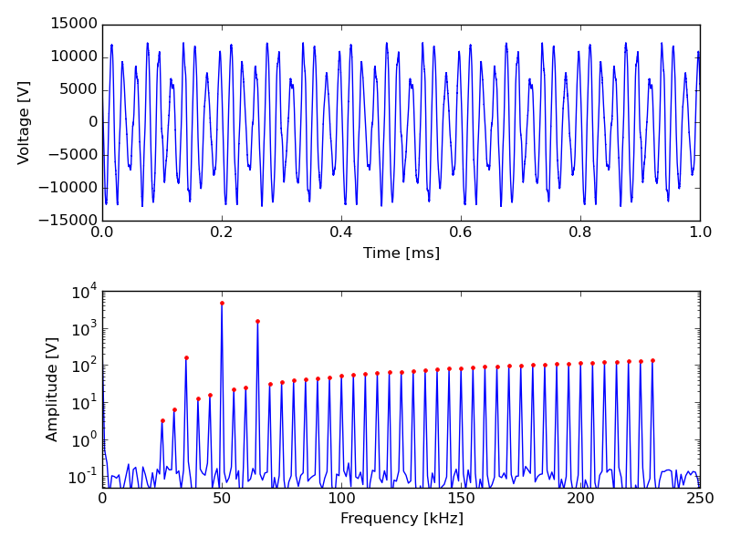
Scripts do not have to be run from the script panel. A stand-alone python script is demonstrated in the example below. The script configures the lockin to make a frequency comb, outputs the comb, measures the comb as a time stream, and plots the measured data in both the time and frequency domain in a figure which is displayed below. Connect OUT 1+ to IN 1+ on the MLA before running this script.
# This script demonstrates some basic features of the MLA API together
# with numpy and matplotlib. The code can be executed line-by-line in a
# python or ipython console, or run as a script with
# "python mla_api_demo.py".
# It will set up the MLA to produce a number of tones and measure
# their response, both in time- and frequency mode. The time mode
# measurement is Fourier transformed and compared with the time mode
# measurement. The result is visualized as a matplotlib plot that should
# appear on screen.

import sys

sys.path.append("PATH TO FOLDER CONTAINING mla_api HERE")

if __name__ == '__main__':  # This line is necessary on Windows operating
    # systems because the MLA is using multiple processes.
    import matplotlib.pyplot as plt
    import numpy as np

    from mlaapi import mla_globals
    from mlaapi import mla_api

    settings = mla_globals.read_config()
    mla = mla_api.MLA(settings)
    mla.connect()
    mla.lockin.start_lockin()
    mla.lockin.set_df(1000)
    mla.lockin.set_frequencies_khz(25 + np.arange(mla.lockin.nr_output_freq) * 5)
    mla.lockin.set_amplitudes(np.arange(1, mla.lockin.nr_output_freq + 1) * 0.0002)
    mla.lockin.set_amplitudes([0.01, 0.3, 0.1], idx=[2, 5, 8])
    mla.lockin.set_output_mask(np.ones(mla.lockin.nr_output_freq))
    mla.osc.start_time_stream(mla.lockin.samples_per_pixel)
    y = mla.osc.get_data(mla.lockin.samples_per_pixel)
    t = np.arange(len(y)) / mla.osc.get_samplerate() * 1e3
    (fig, (ax1, ax2)) = plt.subplots(2, 1)
    ax1.plot(t, y)
    ax1.set_xlabel('Time [ms]')
    ax1.set_ylabel('Voltage [V]')
    y_fft = np.fft.rfft(y) / len(y)
    f_fft_khz = np.fft.rfftfreq(len(y), d=1. / mla.osc.get_samplerate()) * 1e-3
    p = mla.lockin.get_last_pixel()
    a = np.sqrt(p[::2]**2, p[1::2]**2)
    f = mla.lockin.get_frequencies_khz()
    ax2.semilogy(f_fft_khz, abs(y_fft), f, a, '.r')
    ax2.set_xlim([0, 250])
    ax2.set_ylim([5e-2, 1e4])
    ax2.set_xlabel('Frequency [kHz]')
    ax2.set_ylabel('Amplitude [V]')
    fig.tight_layout()
    mla.lockin.stop_lockin()
    mla.disconnect()
    plt.draw()
    plt.show()